Interactive notebook
This tutorial is a Jupyter notebook. You can view it on GitHub or download it to run locally.
Synthetic control for a policy evaluation: two routes to inference#
One state adopts a clean-energy standard in a single quarter, and you want its effect on per-capita renewable electricity generation. There is no clean control group — no other state is a perfect twin of the one that acted. The synthetic control method (Abadie, Diamond & Hainmueller 2010) solves this by building a counterfactual: a weighted blend of untreated “donor” states chosen to track the treated state’s pre-policy trajectory. The post-policy gap between the real state and its synthetic twin is the estimated effect.
The catch: with a single treated unit there is no analytical standard error — in diff-diff, SyntheticControl’s se, t_stat, p_value, and conf_int are NaN by design. Inference instead comes from one of two genuinely different places, and this tutorial walks both:
Philosophy A — compare across regions (permutation): is the treated state’s gap unusual relative to pretending each donor had adopted the policy? This is the in-space placebo (ADH 2010) and the Firpo–Possebom (2018) confidence set.
Philosophy B — compare across time (conformal): Chernozhukov, Wüthrich & Zhu (2021) invert a permutation-over-time test to produce a valid p-value for a hypothesized effect path and a confidence interval for each post-period — something cross-region permutation cannot give.
We generate a synthetic panel where the truth is known, so every diagnostic can be checked against the right answer.
1. The setup#
We use generate_synthetic_control_data, which builds a factor-model panel with one treated unit (id ``0``) and a donor pool. The treated unit’s latent factor loadings and baseline are an exact convex combination of a few donors, so its noiseless trajectory lies in the donor convex hull and a synthetic control can reproduce it closely — the observed fit is approximate because we add transitory and predictor noise (so the pre-period RMSPE is small but not exactly zero). A known
ramping treatment effect (5, 6, 7, 8, 9) is injected into the post period, mimicking a program that scales up as it rolls out.
We use a long pre-period (60 quarters) and a short post-period (5 quarters): synthetic control wants a long, well-matched pre-window, and — as we’ll see in §5 — the conformal average-effect interval needs enough pre-period “blocks” to resolve.
[1]:
%matplotlib inline
import warnings

import matplotlib.pyplot as plt
import numpy as np

from diff_diff import SyntheticControl, generate_synthetic_control_data

# On Apple-Silicon BLAS, harmless "invalid value encountered in matmul" RuntimeWarnings
# can surface from the optimizer; filter only that one (never UserWarnings, which carry
# methodology guidance). See numpy#28687.
warnings.filterwarnings("ignore", category=RuntimeWarning, message=".*encountered in matmul")

panel = generate_synthetic_control_data(
    n_donors=20,
    n_pre=60,
    n_post=5,
    n_factors=3,
    n_predictors=3,
    treatment_effect=5.0,   # first post-period effect
    effect_type="ramp",     # effect grows by effect_growth each post period
    effect_growth=1.0,
    noise_sd=0.6,
    seed=0,
)
print(f"panel: {len(panel)} rows | {panel['unit'].nunique()} units "
      f"(1 treated + 20 donors) | {panel['period'].nunique()} quarters")
panel.head()
panel: 1365 rows | 21 units (1 treated + 20 donors) | 65 quarters
[1]:
| unit | period | outcome | treatment | treat | true_effect | x1 | x2 | x3 | |
|---|---|---|---|---|---|---|---|---|---|
| 0 | 0 | 0 | 49.004867 | 0 | 1 | 0.0 | 0.505192 | -0.399552 | 0.971594 |
| 1 | 0 | 1 | 49.380750 | 0 | 1 | 0.0 | 0.505192 | -0.399552 | 0.971594 |
| 2 | 0 | 2 | 51.031864 | 0 | 1 | 0.0 | 0.505192 | -0.399552 | 0.971594 |
| 3 | 0 | 3 | 50.231137 | 0 | 1 | 0.0 | 0.505192 | -0.399552 | 0.971594 |
| 4 | 0 | 4 | 46.994405 | 0 | 1 | 0.0 | 0.505192 | -0.399552 | 0.971594 |
Columns: unit (0 = the treated state), period (0–59 pre, 60–64 post), outcome (per-capita renewable generation), treatment (absorbing 0/1 — 1 only for the treated state in post quarters), true_effect (the injected effect, for grading), and three pre-treatment covariates x1, x2, x3 — think industrial electricity demand, renewable-resource quality, and installed capacity. SyntheticControl.fit infers the treated unit and the post window directly from
treatment.
2. Fit the synthetic control#
SyntheticControl chooses donor weights (nonnegative, summing to one) so the synthetic state matches the treated state on the predictors, and predictor weights V (via a nested pre-period search) that decide how much each predictor matters. We pass the three covariates as predictors= and use light solver settings to keep the notebook fast.
[2]:
sc = SyntheticControl(
    v_method="nested",
    n_starts=1,
    inner_min_decrease=1e-3,
    optimizer_options={"maxiter": 50},
    seed=0,
)
res = sc.fit(
    panel,
    outcome="outcome",
    treatment="treatment",
    unit="unit",
    time="period",
    predictors=["x1", "x2", "x3"],
)
print(f"ATT (avg post-period gap): {res.att:.3f}")
print(f"pre-period RMSPE:          {res.pre_rmspe:.3f}")
print("\ntop donor weights:")
print(res.get_weights_df().head(5).to_string(index=False))
print("\npredictor weights (V):", {k: round(v, 3) for k, v in res.v_weights.items()})
ATT (avg post-period gap): 6.790
pre-period RMSPE:          0.987

top donor weights:
 unit   weight
    2 0.509414
    3 0.256761
   13 0.081908
   18 0.071077
   16 0.016055

predictor weights (V): {'x1': 0.461, 'x2': 0.081, 'x3': 0.458}
Reading the fit. The synthetic state is a sparse blend — a couple of donors carry most of the weight (here roughly 0.51·unit 2 + 0.26·unit 3 + …). The pre-period RMSPE of about 0.99 is small relative to the 5–9 effect, so the synthetic tracks the treated state closely before the policy. The average post-period gap is ≈ 6.8, against a true average of 7.0.
An honest caveat on the weights. Do not read the weights as “the true recipe.” With many donors and few factors, many weightings reproduce the pre-period path equally well — the weight vector is not identified. What synthetic control identifies is the counterfactual outcome path (and hence the gap/ATT), not a unique set of weights.
[3]:
# Predictor balance: does the synthetic state look like the treated state on the
# covariates? Compare to the raw donor-pool average.
res.predictor_balance.round(3)
[3]:
| predictor | treated | synthetic | donor_mean | |
|---|---|---|---|---|
| 0 | x1 | 0.505 | 0.506 | 0.028 |
| 1 | x2 | -0.400 | -0.363 | 0.298 |
| 2 | x3 | 0.972 | 0.975 | 0.545 |
Balance check. The synthetic state matches the treated state almost exactly on all three covariates (the treated and synthetic columns nearly coincide), while the raw donor_mean is noticeably off. That is the whole point of weighting: a plain average of donors is a poor comparison, but the weighted synthetic is a close one.
[4]:
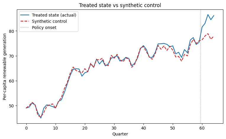
# Plot 1: the treated state vs its synthetic counterfactual.
gd = res.get_gap_df().sort_values("period")
periods = gd["period"].to_numpy()
treated_y = panel[panel["unit"] == 0].sort_values("period")["outcome"].to_numpy()
synth_y = treated_y - gd["gap"].to_numpy()

fig, ax = plt.subplots(figsize=(9, 5))
ax.plot(periods, treated_y, color="#1f77b4", lw=1.8, label="Treated state (actual)")
ax.plot(periods, synth_y, color="#d62728", lw=1.8, ls="--", label="Synthetic control")
ax.axvline(59.5, color="gray", ls=":", lw=1, label="Policy onset")
ax.set_xlabel("Quarter")
ax.set_ylabel("Per-capita renewable generation")
ax.set_title("Treated state vs synthetic control")
ax.legend(loc="upper left")
plt.show()
3. The effect path#
The gap (treated − synthetic) is flat and near zero before the policy and opens up after it. Overlaying the known true_effect shows the estimate recovers the ramp.
[5]:
# Plot 2: estimated gap vs the true effect.
true_eff = panel[panel["unit"] == 0].sort_values("period")["true_effect"].to_numpy()

fig, ax = plt.subplots(figsize=(9, 5))
ax.plot(periods, gd["gap"].to_numpy(), color="#1f77b4", lw=1.8, label="Estimated gap")
ax.plot(periods, true_eff, color="green", lw=1.6, ls=":", label="True effect")
ax.axhline(0, color="black", lw=0.7)
ax.axvline(59.5, color="gray", ls=":", lw=1, label="Policy onset")
ax.set_xlabel("Quarter")
ax.set_ylabel("Gap (treated − synthetic)")
ax.set_title("Estimated effect path")
ax.legend(loc="upper left")
plt.show()
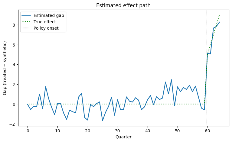
The pre-period gap hugs zero (good fit), and the post-period gap climbs roughly 5 → 9, tracking the truth. But a single treated unit gives us one realization — is this gap distinguishable from noise? That is the inference question, and the rest of the tutorial answers it two ways.
4. Philosophy A — compare across regions#
If the policy did nothing, the treated state’s post/pre RMSPE ratio should look like what we get by pretending each donor was treated. The in-space placebo (ADH 2010 §2.4) refits the synthetic control with each donor cast as the “treated” unit and ranks the real treated state’s ratio against that placebo distribution.
[6]:
placebo = res.in_space_placebo(n_starts=1)
print(f"placebo p-value: {res.placebo_p_value:.4f}")
print(f"treated post/pre RMSPE ratio: {res.rmspe_ratio:.2f} "
      f"(rank 1 of {res.n_placebos + 1})")
placebo p-value: 0.0476
treated post/pre RMSPE ratio: 7.03 (rank 1 of 21)
[7]:
# Plot 3: the placebo distribution of post/pre RMSPE ratios (Abadie's plot).
pl = res.get_placebo_df().sort_values("rmspe_ratio")
colors = ["#d62728" if t else "#bbbbbb" for t in pl["is_treated"]]
labels = ["Treated state" if t else "" for t in pl["is_treated"]]

fig, ax = plt.subplots(figsize=(9, 5))
ax.barh(range(len(pl)), pl["rmspe_ratio"], color=colors)
for y, (lab, t) in enumerate(zip(labels, pl["is_treated"])):
    if t:
        ax.text(pl["rmspe_ratio"].iloc[y], y, "  treated", va="center", color="#d62728")
ax.set_xlabel("Post/pre RMSPE ratio")
ax.set_ylabel("Units (sorted)")
ax.set_title("In-space placebo: the treated state is the most extreme")
ax.set_yticks([])
plt.show()
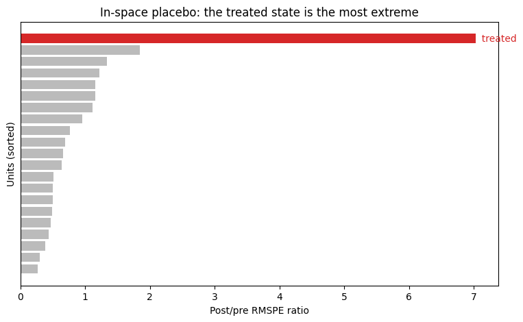
Reading the placebo. The treated state has the largest post/pre RMSPE ratio of all 21 units, giving a permutation p-value of ≈ 0.048 — significant at the 5% level. (With 20 donors the smallest achievable p-value is 1/21; a larger donor pool would give a finer p-value.)
The Firpo–Possebom (2018) confidence set inverts this placebo test over a family of effect paths. The simplest family is a constant effect.
[8]:
cs = res.confidence_set(family="constant", gamma=0.1)
in_set = cs[cs["in_set"]]
print(f"90% confidence set for a constant effect: "
      f"[{in_set['param'].min():.2f}, {in_set['param'].max():.2f}]")
90% confidence set for a constant effect: [4.05, 24.33]
A rigid family. The constant-effect set is wide and lopsided — because our effect ramps rather than staying constant, a single constant value is a poor description, and the test only rejects clearly-wrong constants. This is exactly the gap Philosophy B fills: a per-period interval that needs no parametric effect-path assumption.
First, two standard robustness checks (ADH 2015).
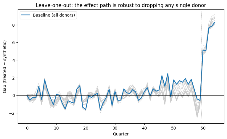
[9]:
# Leave-one-out: drop each weighted donor and refit; how much does the gap move?
loo = res.leave_one_out(n_starts=1)
moved = loo[loo["status"] == "loo"]
print(f"max |change in ATT| when dropping any one donor: {moved['delta_att'].abs().max():.3f}")

# Plot 4: leave-one-out gap paths (spaghetti) around the baseline.
log = res.get_leave_one_out_gaps()
fig, ax = plt.subplots(figsize=(9, 5))
for _, sub in log.groupby("dropped_unit"):
    sub = sub.sort_values("period")
    ax.plot(sub["period"], sub["gap"], color="#cccccc", lw=0.8)
ax.plot(periods, gd["gap"].to_numpy(), color="#1f77b4", lw=2.0, label="Baseline (all donors)")
ax.axhline(0, color="black", lw=0.7)
ax.axvline(59.5, color="gray", ls=":", lw=1)
ax.set_xlabel("Quarter")
ax.set_ylabel("Gap (treated − synthetic)")
ax.set_title("Leave-one-out: the effect path is robust to dropping any single donor")
ax.legend(loc="upper left")
plt.show()
max |change in ATT| when dropping any one donor: 0.761
[10]:
# In-time (backdating) placebo: pretend the policy hit at an earlier quarter and
# check that no "effect" appears before the real onset.
itp = res.in_time_placebo(placebo_periods=[20, 35, 50], n_starts=1)
print(itp[["placebo_period", "placebo_att", "status"]].round(3).to_string(index=False))

# Plot 5: backdated gap paths stay near zero.
itg = res.get_in_time_placebo_gaps()
fig, ax = plt.subplots(figsize=(9, 5))
for pp, sub in itg.groupby("placebo_period"):
    sub = sub.sort_values("period")
    ax.plot(sub["period"], sub["gap"], lw=1.2, label=f"fake onset @ {pp}")
ax.plot(periods, gd["gap"].to_numpy(), color="#1f77b4", lw=2.0, label="real gap")
ax.axhline(0, color="black", lw=0.7)
ax.axvline(59.5, color="gray", ls=":", lw=1, label="real onset")
ax.set_xlabel("Quarter")
ax.set_ylabel("Gap (treated − synthetic)")
ax.set_title("In-time placebo: no effect appears before the real policy")
ax.legend(loc="upper left", fontsize=8)
plt.show()
 placebo_period  placebo_att status
             20        0.598    ran
             35        0.075    ran
             50       -0.367    ran
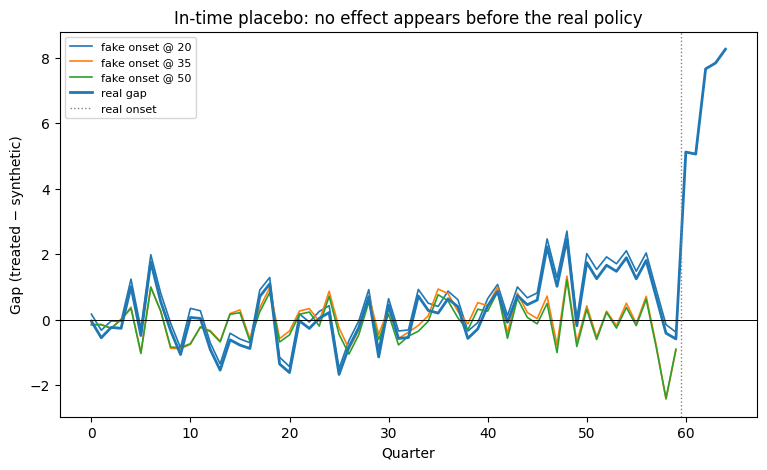
Robustness. Dropping any single donor moves the ATT by at most ≈ 0.76 — the result does not hinge on one comparison state. And backdating the “policy” to earlier quarters produces near-zero placebo effects (all |·| < 1), versus the real 5–9: the divergence is specific to the actual onset, not a pre-existing trend.
5. Philosophy B — compare across time (conformal)#
Philosophy A asks whether the treated state is unusual among units. Conformal inference (CWZ 2021) asks a different question: given this state’s own time series, is the post-period gap distinguishable from the pre-period fluctuations, period by period?
Under a hypothesized effect path, CWZ subtracts it off, fits a time-symmetric proxy synthetic control (constrained least squares on the raw outcomes over all periods — no V matrix; this is what the exactness theory requires, and it differs slightly from the headline ADH fit), and permutes the residuals over time. We start with the sharp null of no effect.
[11]:
joint = res.conformal_test(0.0)
print(f"joint conformal test, H0: no effect  ->  p = {joint['p_value']:.4f} "
      f"(|Pi| = {joint['n_perms']} permutations)")

# Sanity: the test should NOT reject the true ramp.
true_ramp = (
    panel[(panel["unit"] == 0) & (panel["treatment"] == 1)]
    .sort_values("period")["true_effect"].to_numpy()
)
print(f"joint conformal test, H0: the TRUE ramp  ->  p = "
      f"{res.conformal_test(true_ramp)['p_value']:.3f}")
joint conformal test, H0: no effect  ->  p = 0.0154 (|Pi| = 65 permutations)
joint conformal test, H0: the TRUE ramp  ->  p = 0.831
The sharp null of no effect is rejected (p ≈ 0.015), while the true ramp is not rejected (large p) — exactly as it should be. Now the payoff: a confidence interval for the effect in each post quarter, by inverting that test over a grid of candidate values.
[12]:
ci = res.conformal_confidence_intervals(alpha=0.1, scheme="moving_block")
ci_show = ci[["period", "lower", "upper"]].copy()
ci_show["true_effect"] = true_eff[-5:]
print(ci_show.round(2).to_string(index=False))
 period  lower  upper  true_effect
     60   3.91   5.87          5.0
     61   4.50   6.46          6.0
     62   6.56   8.52          7.0
     63   7.45   9.52          8.0
     64   7.94  10.01          9.0
[13]:
# Plot 6: the per-period conformal CI band (the payoff).
post_periods = ci["period"].to_numpy()
sc_gap_post = gd[gd["phase"] == "post"].sort_values("period")["gap"].to_numpy()

fig, ax = plt.subplots(figsize=(9, 5))
ax.fill_between(post_periods, ci["lower"], ci["upper"], alpha=0.25, color="#1f77b4",
                label="90% conformal CI")
ax.plot(post_periods, sc_gap_post, "s--", color="#1f77b4", label="SC gap (point estimate)")
ax.plot(post_periods, true_eff[-5:], "o-", color="green", label="True effect")
ax.set_xlabel("Quarter")
ax.set_ylabel("Effect on per-capita generation")
ax.set_title("CWZ pointwise conformal intervals track the ramping effect")
ax.legend(loc="upper left")
plt.show()
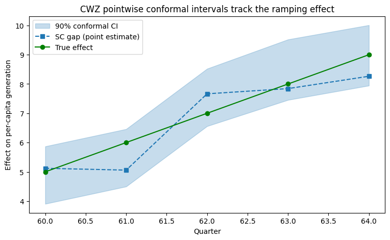
Reading the band. Each post quarter gets its own 90% interval, and the band rises with the ramp, containing the true effect in every period — without ever assuming the effect is constant or linear. This is what cross-region permutation could not deliver: a calibrated, period-by-period uncertainty statement. (Each interval is a 90% interval, so an occasional period legitimately missing the truth would be expected; here all five contain it.)
For a single-number summary, CWZ also gives a confidence interval for the average effect by collapsing the panel into non-overlapping blocks.
[14]:
ae = res.conformal_average_effect(alpha=0.1, scheme="moving_block")
print(f"90% CI for the average post-period effect: "
      f"[{ae['lower']:.2f}, {ae['upper']:.2f}]  (true average = 7.0)")
print(f"(collapsed into {ae['n_blocks']} blocks)")
90% CI for the average post-period effect: [6.50, 7.48]  (true average = 7.0)
(collapsed into 13 blocks)
The average-effect interval is ≈ [6.5, 7.5] — tight, bounded, and bracketing the true 7.0. Practitioner footnote: this interval works by collapsing the panel into T/T* = 13 blocks and permuting them; its resolution is 1/13 ≈ 0.077, comfortably below α = 0.1. With a short pre-period the block count drops, the permutation grid coarsens, and the interval can become uninformative (the method fails closed to (-∞, ∞) rather than reporting a falsely-precise width). That is
precisely why we used a long, 60-quarter pre-window.
6. The two philosophies, side by side#
Philosophy A (across regions) |
Philosophy B (across time) |
|
|---|---|---|
Question |
Is the treated unit unusual vs other units? |
Is the gap unusual vs this unit’s own history? |
Tools |
in-space placebo, Firpo–Possebom set |
CWZ test, pointwise CIs, average-effect CI |
Resolution set by |
number of donors ( |
number of periods / blocks |
Output |
one p-value; a set for a constant/linear family |
per-period intervals; a free-form path p-value |
Needs |
a sizable donor pool |
a long pre-period |
Neither dominates. Cross-region permutation is the classic, intuitive check and is robust to how the within-unit errors are correlated. Over-time conformal is the only one of the two that gives you a calibrated interval for each period’s effect without assuming a parametric shape — invaluable when, as here, the effect evolves.
7. Practitioner takeaways#
Reach for synthetic control when a single (or a few) units are treated and no untreated unit is a credible stand-alone control, but a weighted blend of donors can reproduce the treated unit’s pre-period path. Check the pre-period RMSPE and the predictor-balance table before trusting any post-period gap.
Don’t over-read the weights — the counterfactual path is identified; the exact weights are not.
For inference, use both routes. Report the in-space placebo p-value and a robustness pair (leave-one-out + in-time placebo); add CWZ pointwise intervals when stakeholders need period-by-period uncertainty, and the average-effect interval for a headline number.
Design for the method you’ll use: cross-region permutation wants a sizable donor pool (the p-value floor is
1/(J+1)); conformal inference — especially the average-effect interval — wants a long pre-period.
Extensions not covered here: folding covariates into the conformal proxy; the q = 2/ q = ∞ conformal norms (we used q = 1); the scheme="iid" permutation set; and the cv/ inverse_variance routes for selecting V.
Related tutorials: 03 — Synthetic DiD (a regression-weighted cousin) and 10 — TROP (a triply-robust panel estimator).
References: Abadie, Diamond & Hainmueller (2010, 2015); Firpo & Possebom (2018); Chernozhukov, Wüthrich & Zhu (2021). Full citations in the project references.