Interactive notebook
This tutorial is a Jupyter notebook. You can view it on GitHub or download it to run locally.
When the Average Hides the Action - Distributional DiD with Changes-in-Changes#
A loyalty program was rolled out to a lower-spend customer segment. Finance ran the standard difference-in-differences on monthly spend and got a flat zero - the program looks dead, and leadership is ready to kill it. This tutorial shows how Changes-in-Changes (CiC) - the distributional DiD estimator of Athey & Imbens
reveals that the program in fact worked exactly where it was aimed: it moved the bottom half of the spend distribution, which the mean cannot see under this much top-end variance.
What you’ll learn
When to reach for CiC instead of (or alongside) mean DiD and the staggered estimators.
How to read a quantile-treatment-effect (QTE) profile, and how to make joint “which quantiles moved” claims with sup-t uniform bands.
What the interior point-identification range guardrail does when support is short.
CiC’s headline robustness property: its distributional answer does not depend on whether you analyze levels or logs - and why that is not true for mean DiD or for the quantile-DiD (QDiD) comparison estimator.
How to adjust for covariate-composition differences with the quantile-regression covariate branch (
covariates=), and what the conditional support diagnostic guards.Where to go next with
practitioner_next_steps().
When is CiC the right tool?#
The decision comes down to the design and the question:
Two groups, two periods (2x2), and a distributional question - “who moved, not just how much on average?” - use ChangesInChanges. It estimates the treated group’s full counterfactual outcome distribution, so you get an ATT and quantile treatment effects on one bootstrap.
Mean-only question, trustworthy parallel trends on your chosen scale - plain
DifferenceInDifferencesis simpler and faster.Staggered adoption across many periods - CiC does not apply (it is 2x2 only); use
CallawaySantAnnaor another heterogeneity-robust estimator for mean effects.QDiD is the quantile-by-quantile DiD comparison estimator. Athey & Imbens (2006, p. 447) recommend CiC over it - the levels-vs-logs section makes their reason concrete on our data.
Our setting is a genuine 2x2 with repeated cross-sections: a fresh sample of customers is drawn each period (typical for transaction panels). CiC also supports true panels - panel=True changes only the bootstrap resampling scheme (unit-block instead of pooled rows), not the point estimator.
[1]:
import matplotlib.pyplot as plt
import numpy as np
import pandas as pd
from scipy import stats

from diff_diff import ChangesInChanges, DifferenceInDifferences, QDiD, practitioner_next_steps
The data#
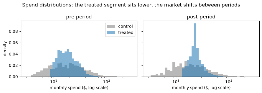
We simulate the program so that the truth is known by construction - every claim below can be checked against it. Three ingredients, each realistic on its own:
Heavy-tailed spend. Customer spend is lognormal-ish: median about $30, a long right tail past $200. The tail is what makes the mean a noisy summary.
A nonlinear market trend. Between periods the whole market moves by a smooth transformation with
log y_post = ALPHA + GAMMA * log y_preandGAMMA = 1.06: premium spend grows faster than budget spend. Dollar trends are therefore not parallel across differently-composed groups - and neither are log trends.A targeted program. The treated group is a lower-spend loyalty segment, and the program lift fades smoothly - a logistic in spend rank - from about +65% for near-lapsed customers to effectively zero across the segment’s upper half. The true mean effect on the treated is $3.01.
The seed is locked so every number in the prose is reproducible; a companion drift test re-derives them against the installed library.
[2]:
SEED = 27
N_CELL = 901  # 17*53 - coprime to 20 (quantile grid) and 100 (QR tau grid)

MU_LOG, SIGMA_LOG = 3.4, 0.75  # log-spend location/scale: median spend ~ $30
GAMMA, ALPHA = 1.06, -0.17  # market trend: log y_post = ALPHA + GAMMA * log y_pre
U_LO, U_HI = 0.05, 0.90  # loyalty segment spans the interior of the spend distribution
BETA_A, BETA_B = 1.2, 2.2  # segment tilt toward lower spenders
LIFT_MAX, LIFT_MID, LIFT_SCALE = 0.65, 0.22, 0.07  # program lift, strongest for near-lapsed


def h_pre(u):
    return np.exp(MU_LOG + SIGMA_LOG * stats.norm.ppf(u))


def h_post(u):
    return np.exp(ALPHA + GAMMA * (MU_LOG + SIGMA_LOG * stats.norm.ppf(u)))


def lift(u):
    return LIFT_MAX / (1.0 + np.exp((u - LIFT_MID) / LIFT_SCALE))


def make_spend_data(seed=SEED, n=N_CELL):
    rng = np.random.default_rng(seed)
    u00 = rng.uniform(0.0005, 0.9995, n)
    u01 = rng.uniform(0.0005, 0.9995, n)
    u10 = U_LO + (U_HI - U_LO) * rng.beta(BETA_A, BETA_B, n)
    u11 = U_LO + (U_HI - U_LO) * rng.beta(BETA_A, BETA_B, n)
    frames = []
    for g, t, y in (
        (0, 0, h_pre(u00)),
        (0, 1, h_post(u01)),
        (1, 0, h_pre(u10)),
        (1, 1, h_post(u11) * (1.0 + lift(u11))),
    ):
        frames.append(pd.DataFrame({"treated": g, "post": t, "spend": y}))
    return pd.concat(frames, ignore_index=True)


df = make_spend_data()
y00 = df.query("treated == 0 and post == 0")["spend"].to_numpy()
y10 = df.query("treated == 1 and post == 0")["spend"].to_numpy()
y11 = df.query("treated == 1 and post == 1")["spend"].to_numpy()

print(f"{len(df)} rows ({N_CELL} per group x period cell)")
print(f"control pre-period spend:  median ${np.median(y00):.2f}, mean ${y00.mean():.2f}")
print(f"treated pre-period spend:  median ${np.median(y10):.2f}  (lower-spend segment)")
3604 rows (901 per group x period cell)
control pre-period spend:  median $31.03, mean $39.79
treated pre-period spend:  median $20.86  (lower-spend segment)
[3]:
fig, axes = plt.subplots(1, 2, figsize=(9, 3.2), sharey=True)
bins = np.geomspace(3, 300, 45)
for ax, period, label in ((axes[0], 0, "pre-period"), (axes[1], 1, "post-period")):
    for g, color, name in ((0, "tab:gray", "control"), (1, "tab:blue", "treated")):
        vals = df.query(f"treated == {g} and post == {period}")["spend"]
        ax.hist(vals, bins=bins, density=True, alpha=0.55, color=color, label=name)
    ax.set_xscale("log")
    ax.set_xlabel("monthly spend ($, log scale)")
    ax.set_title(label)
axes[0].set_ylabel("density")
axes[0].legend()
fig.suptitle("Spend distributions: the treated segment sits lower, the market shifts between periods")
fig.tight_layout()
plt.show()
The mean answer#
Standard practice first: difference-in-differences on mean spend, with robust standard errors.
[4]:
did = DifferenceInDifferences().fit(df, outcome="spend", treatment="treated", time="post")
print(did.summary())
======================================================================
             Difference-in-Differences Estimation Results
======================================================================

Observations:                   3604
Treated:                        1802
Control:                        1802
R-squared:                    0.0939
Variance:                            HC1 heteroskedasticity-robust

----------------------------------------------------------------------
Parameter           Estimate    Std. Err.     t-stat      P>|t|
----------------------------------------------------------------------
ATT                   0.2178       1.7351      0.126     0.9001
----------------------------------------------------------------------

95% Confidence Interval: [-3.1841, 3.6197]
CV (SE/abs(ATT)):             7.9670

Signif. codes: '***' 0.001, '**' 0.01, '*' 0.05, '.' 0.1
======================================================================
The mean verdict: ATT = $0.22, p = 0.90, confidence interval [-$3.18, $3.62]. By this reading the program did nothing, and it gets killed.
Two things are wrong with that reading, and only one of them is about power:
Noise: the long spend tail puts the DiD standard error near $1.74, so even the true $3.01 mean effect would be hard to detect.
Bias: the market trend is multiplicative (
GAMMA = 1.06), so dollar trends are not parallel between a $21-median segment and a $31-median control group. Mean DiD with these groups does not target the truth on this scale in the first place - the $0.22 is not an unlucky draw around $3.01.
CiC was built for exactly this situation: it never assumes additive-in-levels trends.
Changes-in-Changes: the full picture#
CiC (Athey & Imbens 2006) treats the control group’s period-to-period change as a transformation of the whole distribution and applies that transformation to the treated group’s pre-period distribution. Formally, the counterfactual outcome distribution is \(F_{10}(F_{00}^{-1}(F_{01}(y)))\) (their Theorem 3.1): “give every treated customer the outcome move that a control customer at the same rank experienced.” Identification needs a monotone outcome model in a scalar unobservable and time-invariance of that unobservable within groups - not parallel mean trends (more on that in the levels-vs-logs section).
Inference is bootstrap-only (999 replicates here, seeded). The point estimates match the R qte package exactly; see the methodology registry for the parity details.
[5]:
cic = ChangesInChanges(n_bootstrap=999, seed=SEED).fit(
    df, outcome="spend", treatment="treated", time="post"
)
print(cic.summary())
========================================================================================
                    Changes-in-Changes (Athey & Imbens 2006) Results
========================================================================================
Observations: 3604    Mode: repeated cross-section
Cells: control pre=901, control post=901, treated pre=901, treated post=901
Inference: bootstrap (999/999 valid replicates), replicate-SD SEs, normal-approximation intervals
Point-identified interior quantile range (eq. 17): (0.0000, 1.0000)
----------------------------------------------------------------------------------------
              Estimate     Std.Err         t     P>|t|  [95% Conf. Int.]
----------------------------------------------------------------------------------------
       ATT      3.0476      1.0628      2.87     0.004  [   0.9646,    5.1306] **

Quantile treatment effects:
----------------------------------------------------------------------------------------
      0.05      4.9087      0.8252      5.95     0.000  [   3.2914,    6.5260] ***
      0.10      5.4037      0.9124      5.92     0.000  [   3.6154,    7.1920] ***
      0.15      5.4575      0.9586      5.69     0.000  [   3.5787,    7.3364] ***
      0.20      5.3724      0.8286      6.48     0.000  [   3.7483,    6.9965] ***
      0.25      5.4433      0.8918      6.10     0.000  [   3.6953,    7.1913] ***
      0.30      5.5808      1.0359      5.39     0.000  [   3.5504,    7.6112] ***
      0.35      4.2059      1.0267      4.10     0.000  [   2.1936,    6.2181] ***
      0.40      4.1270      0.9387      4.40     0.000  [   2.2871,    5.9668] ***
      0.45      4.1575      0.8804      4.72     0.000  [   2.4318,    5.8831] ***
      0.50      3.8598      1.1207      3.44     0.001  [   1.6632,    6.0564] ***
      0.55      2.9191      1.4494      2.01     0.044  [   0.0782,    5.7599] *
      0.60      1.7319      1.3488      1.28     0.199  [  -0.9116,    4.3755]
      0.65      0.7939      1.4164      0.56     0.575  [  -1.9821,    3.5699]
      0.70      0.3729      1.5852      0.24     0.814  [  -2.7341,    3.4799]
      0.75      0.5906      1.5996      0.37     0.712  [  -2.5447,    3.7258]
      0.80      1.3649      1.6163      0.84     0.398  [  -1.8030,    4.5327]
      0.85      1.0424      2.4456      0.43     0.670  [  -3.7510,    5.8357]
      0.90     -0.3910      2.3746     -0.16     0.869  [  -5.0450,    4.2631]
      0.95      2.7981      3.3682      0.83     0.406  [  -3.8035,    9.3997]
========================================================================================
Signif. codes: *** p<0.001, ** p<0.01, * p<0.05
[6]:
qe = cic.quantile_effects

# The DGP is synthetic, so the true QTE curve is computable by Monte Carlo:
rng_mc = np.random.default_rng(123456)
u_mc = U_LO + (U_HI - U_LO) * rng_mc.beta(BETA_A, BETA_B, 2_000_000)
truth = np.quantile(h_post(u_mc) * (1 + lift(u_mc)), cic.quantiles) - np.quantile(
    h_post(u_mc), cic.quantiles
)

fig, ax = plt.subplots(figsize=(7.5, 4))
ax.fill_between(qe["quantile"], qe["conf_low"], qe["conf_high"], alpha=0.25,
                color="tab:blue", label="pointwise 95% CI")
ax.plot(qe["quantile"], qe["qte"], "o-", color="tab:blue", label="CiC QTE")
ax.plot(cic.quantiles, truth, "--", color="black", alpha=0.7,
        label="true effect (known by construction)")
ax.axhline(0, color="gray", lw=1)
ax.axhline(did.att, color="tab:red", lw=1.2, ls=":", label=f"mean DiD (${did.att:.2f})")
ax.set_xlabel("spend quantile (tau)")
ax.set_ylabel("treatment effect ($)")
ax.set_title("The program moved the bottom of the distribution, not the mean")
ax.legend(loc="upper right")
fig.tight_layout()
plt.show()
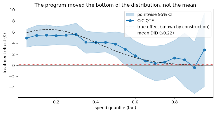
The QTE profile tells the real story: +$4.91 at the 5th percentile, +$5.44 at the 25th, +$3.86 at the median, and nothing distinguishable from zero above the 70th. For a $15-25/month customer, a $5 lift is a 20-30% change - the program reactivated near-lapsed customers, exactly its design goal.
Note the headline ATT: $3.05 (p = 0.004), right on the $3.01 truth - CiC’s mean is the mean of a correctly constructed counterfactual distribution, so it does not inherit mean DiD’s nonparallel-dollar-trend bias. Same data, same 2x2, two very different answers - and here the distributional one is right by construction.
Which quantiles moved? Joint claims and the interior range#
Reading 19 pointwise confidence intervals off the plot and declaring “significant below the median” is a multiple-testing mistake - pointwise intervals over-reject when read jointly. For joint statements use uniform_bands(): simultaneous sup-t bands over the whole grid, computed at the qte package’s fixed 95% level (the band level deliberately does not follow alpha; that is the parity convention).
[7]:
bands = cic.uniform_bands()
excluded = (bands["band_low"] > 0) | (bands["band_high"] < 0)
sig = [f"{t:.2f}" for t, e in zip(cic.quantiles, excluded) if e]
print(f"sup-t critical value: {cic.sup_t_crit:.3f}")
print(f"quantiles whose uniform band excludes zero: {sig}")

fig, ax = plt.subplots(figsize=(7.5, 4))
ax.fill_between(qe["quantile"], qe["conf_low"], qe["conf_high"], alpha=0.25,
                color="tab:blue", label="pointwise 95% CI")
ax.plot(bands["quantile"], bands["band_low"], "-", color="tab:purple", lw=1.2,
        label="sup-t uniform band (95%)")
ax.plot(bands["quantile"], bands["band_high"], "-", color="tab:purple", lw=1.2)
ax.plot(qe["quantile"], qe["qte"], "o-", color="tab:blue", label="CiC QTE")
ax.axhline(0, color="gray", lw=1)
ax.set_xlabel("spend quantile (tau)")
ax.set_ylabel("treatment effect ($)")
ax.set_title("Joint claim: the bands exclude zero for every quantile up to the median")
ax.legend(loc="upper right")
fig.tight_layout()
plt.show()
sup-t critical value: 3.260
quantiles whose uniform band excludes zero: ['0.05', '0.10', '0.15', '0.20', '0.25', '0.30', '0.35', '0.40', '0.45', '0.50']
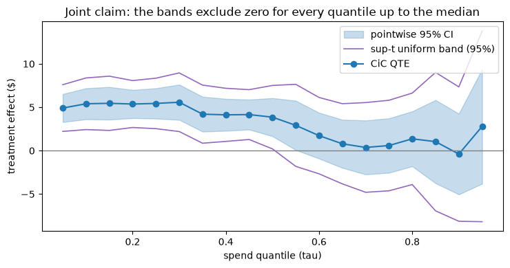
The joint statement survives: the uniform bands exclude zero for every grid quantile from 0.05 through 0.50, and for none above - so “the program lifted the bottom half of the spend distribution” holds as a single, simultaneous claim.
Be precise about what the bands say above the median: they are silent, not exonerating. Non-exclusion of zero is absence of evidence, not evidence of absence - on real data you would report “no detectable effect above the median”, never “zero effect”. (Notice the pointwise row at tau = 0.55: nominally significant at p = 0.044. That is exactly the kind of isolated pointwise blip that evaporates under the joint bands - chasing it would be the multiple-testing mistake this section is about. Here we happen to know the truth is ~0 above the median by construction.)
The interior-range guardrail. CiC quantile effects are point-identified only strictly inside an interior range \((q_{lower}, q_{upper})\) - eq. (17) of the paper - determined by where the treated pre-period distribution sits inside the control pre-period support. Our sample is support-clean, so the range is the trivial \((0, 1)\) and every grid quantile is interior. But short support is common in practice - suppose the control sample had only covered mid-market customers. CiC does not fail silently: watch the warnings this variant raises, and what happens to the tail inference.
[8]:
def make_midmarket_variant(seed=SEED, n=N_CELL):
    # Same market, same program - but the control SAMPLE only covers
    # mid-market customers (spend ranks 15%-85%).
    rng = np.random.default_rng(seed + 1)
    u00 = rng.uniform(0.15, 0.85, n)
    u01 = rng.uniform(0.15, 0.85, n)
    u10 = U_LO + (U_HI - U_LO) * rng.beta(BETA_A, BETA_B, n)
    u11 = U_LO + (U_HI - U_LO) * rng.beta(BETA_A, BETA_B, n)
    frames = []
    for g, t, y in (
        (0, 0, h_pre(u00)),
        (0, 1, h_post(u01)),
        (1, 0, h_pre(u10)),
        (1, 1, h_post(u11) * (1.0 + lift(u11))),
    ):
        frames.append(pd.DataFrame({"treated": g, "post": t, "spend": y}))
    return pd.concat(frames, ignore_index=True)


cic_v = ChangesInChanges(n_bootstrap=999, seed=SEED).fit(
    make_midmarket_variant(), outcome="spend", treatment="treated", time="post"
)
print(f"interior range: ({cic_v.q_lower:.4f}, {cic_v.q_upper:.4f})")
print("\nquantiles outside the interior range (point estimates kept, inference NaN):")
print(cic_v.quantile_effects[cic_v.quantile_effects["se"].isna()].to_string(index=False))
interior range: (0.1698, 0.9956)

quantiles outside the interior range (point estimates kept, inference NaN):
 quantile      qte  se  t_stat  p_value  conf_low  conf_high
     0.05 2.726330 NaN     NaN      NaN       NaN        NaN
     0.10 4.696848 NaN     NaN      NaN       NaN        NaN
     0.15 6.264059 NaN     NaN      NaN       NaN        NaN
diff_diff/changes_in_changes.py:981: UserWarning: Treated pre-period outcomes fall outside the control pre-period support (Athey-Imbens Assumption 3.4 violated). The counterfactual distribution is only partially identified (Corollary 3.1): quantile effects are reliable only inside the reported (q_lower, q_upper) interior range, and the ATT involves extrapolation at the support edges.
  _check_support(cells)
diff_diff/changes_in_changes.py:1324: UserWarning: Quantile effects at [0.05, 0.1, 0.15] lie outside the point-identified interior range (0.1698, 0.9956) (Athey-Imbens eq. 17 / Theorem 5.3). Point estimates are reported for qte parity, but their inference fields are set to NaN.
  return _fit_distributional(
Two warnings fired, on purpose and loudly: treated customers fall outside the control sample’s support (Athey-Imbens Assumption 3.4), and the quantiles at 0.05-0.15 lie outside the resulting interior range (0.17, 0.996). Those tail effects keep their point estimates (matching the R qte package) but report NaN inference - the estimator refuses to hand you confidence intervals for quantiles where the counterfactual is extrapolated. If you see these warnings on real data, fix the sampling
frame or report the interior range alongside the tails.
Scale is not a nuisance: levels, logs, and why CiC doesn’t care#
Every mean-DiD practitioner has faced the question: levels or logs? Parallel trends on one scale generally fails on the other, so the modeling choice changes the answer. On our data it changes the answer completely:
[9]:
df_log = df.assign(log_spend=np.log(df["spend"]))
did_log = DifferenceInDifferences().fit(
    df_log, outcome="log_spend", treatment="treated", time="post"
)
print(f"DiD on spend ($):    ATT = {did.att:+.2f}   (p = {did.p_value:.3f})  -> 'no effect'")
print(
    f"DiD on log(spend):   ATT = {did_log.att:+.4f}  (p = {did_log.p_value:.4f})"
    f"  -> '+{100 * (np.exp(did_log.att) - 1):.1f}% - big win'"
)
DiD on spend ($):    ATT = +0.22   (p = 0.900)  -> 'no effect'
DiD on log(spend):   ATT = +0.1307  (p = 0.0011)  -> '+14.0% - big win'
Same data: $0.22 (p = 0.90) in dollars, +14.0% (p = 0.001) in logs. Neither scale has parallel trends here (the market trend is y -> e^ALPHA * y^GAMMA, which is additive in neither dollars nor logs across differently-composed groups), so neither number should be trusted - but nothing in the output tells you that. The scale choice silently is the identification assumption.
CiC removes that choice from the table. Its identifying assumptions - a monotone outcome model and time-invariant unobservables - are statements about ranks, so they are unchanged by any strictly increasing transformation. For unconditional fits the estimated counterfactual distribution is equivariant: fit in dollars or fit in logs, and you get the same answer mapped through the transformation. Concretely, the counterfactual quantiles from the levels fit equal exp() of the
counterfactual quantiles from the log fit, up to floating-point rounding:
[10]:
cic_log = ChangesInChanges(n_bootstrap=0).fit(
    df_log, outcome="log_spend", treatment="treated", time="post"
)

# Counterfactual quantiles = treated-post quantiles minus the QTE. CiC's internal
# quantile convention is R type-1 (an order statistic - no interpolation), which
# numpy calls "inverted_cdf". Order statistics commute with monotone transforms,
# and no n*tau lands on an integer (901 is coprime to 20), so the identity is
# exact up to the exp/log round-trip:
grid = cic.quantiles
q11_lvl = np.quantile(y11, grid, method="inverted_cdf")
q11_log = np.quantile(np.log(y11), grid, method="inverted_cdf")
cf_levels_fit = q11_lvl - cic.quantile_effects["qte"].to_numpy()
cf_log_fit = np.exp(q11_log - cic_log.quantile_effects["qte"].to_numpy())

comparison = pd.DataFrame(
    {"tau": grid, "cf_from_levels_fit": cf_levels_fit, "cf_from_log_fit": cf_log_fit}
)
print(comparison.iloc[[2, 9, 14, 18]].to_string(index=False))
max_rel = np.max(np.abs(cf_levels_fit - cf_log_fit) / cf_levels_fit)
print(f"\nmax relative difference across all 19 quantiles: {max_rel:.2e}")
 tau  cf_from_levels_fit  cf_from_log_fit
0.15           13.902084        13.902084
0.50           20.316616        20.316616
0.75           29.905258        29.905258
0.95           45.271539        45.271539

max relative difference across all 19 quantiles: 0.00e+00
The two fits agree to floating-point precision (the only daylight is the exp/log round-trip, at most a few units in the last bit - on this machine it is exactly zero). The levels-vs-logs debate simply does not arise for CiC’s distributional answer. (The scope matters: this exact equivariance holds for unconditional fits - the covariate branch below runs linear quantile regressions, which are not equivariant to nonlinear transforms. And means never commute with transforms, so the ATT is
scale-specific for every estimator, CiC included.)
QDiD does not have this property, and that is the substance of Athey & Imbens’s recommendation (p. 447): QDiD imposes the additive quantile-DiD model on whatever scale you happen to fit, so its answer shifts with the scale:
[11]:
qdid = QDiD(n_bootstrap=0).fit(df, outcome="spend", treatment="treated", time="post")
qdid_log = QDiD(n_bootstrap=0).fit(
    df_log, outcome="log_spend", treatment="treated", time="post"
)

# Back-transform the log-scale QDiD profile to dollars (QDiD's treated-post
# quantiles are R type-7, numpy's default "linear" interpolation):
q11_t7_log = np.quantile(np.log(y11), grid, method="linear")
qdid_backmapped = np.exp(q11_t7_log) - np.exp(q11_t7_log - qdid_log.quantile_effects["qte"].to_numpy())
qdid_gap = qdid.quantile_effects["qte"].to_numpy() - qdid_backmapped

table = pd.DataFrame(
    {
        "tau": grid,
        "QDiD_levels": qdid.quantile_effects["qte"].to_numpy(),
        "QDiD_logs_backmapped": qdid_backmapped,
        "gap": qdid_gap,
        "CiC_levels": cic.quantile_effects["qte"].to_numpy(),
    }
)
print(table.iloc[[4, 9, 14, 17]].round(2).to_string(index=False))
print(f"\nQDiD levels-vs-logs gap: median |gap| = {np.median(np.abs(qdid_gap)):.2f}, "
      f"max |gap| = {np.max(np.abs(qdid_gap)):.2f} (at tau = {grid[np.argmax(np.abs(qdid_gap))]:.2f})")
 tau  QDiD_levels  QDiD_logs_backmapped   gap  CiC_levels
0.25         5.61                  5.61 -0.00        5.44
0.50         2.59                  2.83 -0.24        3.86
0.75        -3.77                 -1.67 -2.10        0.59
0.90        -8.48                 -2.84 -5.65       -0.39

QDiD levels-vs-logs gap: median |gap| = 0.24, max |gap| = 5.65 (at tau = 0.90)
The gap grows toward the top of the distribution - $0.24 at the median, $2.10 at the 75th percentile, $5.65 at the 90th - and worse, QDiD-in-levels reports a loss of $8.48 at the 90th percentile where the truth (and CiC) say zero: its additive dollar model extrapolates the control group’s premium-segment dollar growth onto a treated segment that has no premium customers. Fit QDiD on logs instead and that loss shrinks by two-thirds. An estimator whose story changes with the analyst’s scale choice is a fragile primary; use QDiD as a cross-check beside CiC, not instead of it. (When QDiD’s implied counterfactual quantile curve is non-monotone - another symptom of the same model failure - the fit warns; on this data it stays monotone on both scales.)
When the mix differs: covariates#
CiC’s time-invariance assumption can fail observably: if the treated and control groups differ in composition on a variable that also drives the period-to-period trend, the unconditional counterfactual attributes the wrong trend to the treated group. The fix is to condition: covariates= runs the comparison within covariate values (per-cell linear quantile regressions on a 99-tau grid - an exact port of the R qte package’s xformla branch, including its conditional-rank
imputation).
Here is a second program where that matters. The outcome is an engagement index; the treated group skews toward longer-tenure customers (+0.8 years on average), and this quarter’s organic engagement growth is strongly tenure-driven while tenure’s level link is weak - latent-index slopes 0.6 (trend) vs 0.15 (level), which the x8 index scaling turns into 4.8 vs 1.2 engagement points per tenure-year. That trend/level decoupling is what makes the confounding bite. The
program’s true effect is 6.0 points, constant for everyone.
[12]:
COV_SEED, COV_N = 272, 299  # cell size coprime to 100 (QR tau grid)
COV_EFFECT = 6.0  # true program effect, engagement points
COV_SHIFT, COV_TREND, COV_LEVEL, COV_SCALE = 0.8, 0.6, 0.15, 8.0


def make_engagement_data(seed=COV_SEED, n=COV_N):
    rng = np.random.default_rng(seed)
    frames = []
    for g in (0, 1):
        for t in (0, 1):
            x = rng.uniform(0, 2, n) + COV_SHIFT * g  # tenure (years, centered scale)
            noise = rng.normal(0, 0.4, n)
            y = COV_SCALE * (0.5 + COV_LEVEL * x + COV_TREND * x * t + noise) + COV_EFFECT * g * t
            frames.append(pd.DataFrame({"treated": g, "post": t, "tenure": x, "engagement": y}))
    return pd.concat(frames, ignore_index=True)


eng = make_engagement_data()

cic_unc = ChangesInChanges(n_bootstrap=999, seed=SEED).fit(
    eng, outcome="engagement", treatment="treated", time="post"
)
# The covariate branch refits every per-cell quantile regression inside every
# bootstrap replicate - this cell takes about a minute:
cic_cov = ChangesInChanges(n_bootstrap=99, seed=SEED).fit(
    eng, outcome="engagement", treatment="treated", time="post", covariates=["tenure"]
)

print(f"true effect:        {COV_EFFECT:.1f} points")
print(f"unconditional CiC:  ATT = {cic_unc.att:.2f}  "
      f"CI [{cic_unc.conf_int[0]:.2f}, {cic_unc.conf_int[1]:.2f}]")
print(f"conditional CiC:    ATT = {cic_cov.att:.2f}  "
      f"CI [{cic_cov.conf_int[0]:.2f}, {cic_cov.conf_int[1]:.2f}]   (covariates=['tenure'])")
true effect:        6.0 points
unconditional CiC:  ATT = 9.38  CI [8.32, 10.45]
conditional CiC:    ATT = 6.53  CI [5.35, 7.70]   (covariates=['tenure'])
The unconditional fit reports 9.38 with CI [8.32, 10.45] - confidently wrong, because the tenure-driven trend is not a monotone transformation of the outcome (the trend/level decoupling is what breaks the unconditional assumption). Conditioning on tenure brings the estimate to 6.53 with CI [5.35, 7.70], covering the truth.
Practical notes for the covariate branch:
Covariates must be numeric (dummy-encode categoricals first).
A conditional support diagnostic replaces the interior-range guardrail: if more than 10% of treated pre-period outcomes fall outside their conditional quantile envelope, a warning flags out-of-support extrapolation (Melly & Santangelo 2015, Assumption 4). This fit is clean, so no warning fired.
Bootstrap cost scales with the quantile-regression refits - budget minutes, not seconds, at larger sizes (the same cost profile as the R
qtepackage).
What next#
Fitted results know their own follow-up work: practitioner_next_steps() reads the estimator type, covariate status, and bootstrap health, and returns the remaining steps of the Baker, Callaway, Cunningham, Goodman-Bacon & Sant’Anna (2025) workflow, with runnable snippets that mirror this fit’s exact specification.
[13]:
guidance = practitioner_next_steps(cic)
============================================================
Practitioner Guidance — ChangesInChanges (CiC)
Baker et al. (2025) 8-Step Workflow
============================================================

Recommended next steps (9 remaining):

  * [HIGH] Step 1: Define target parameter
    Why: State explicitly what causal effect you are estimating (ATT, ATT(g,t), weighted/unweighted) and what policy question it answers.
    >>> # What is the target parameter? ATT? Weighted or unweighted?

  * [HIGH] Step 2: State identification assumptions (distributional)
    Why: Name the distributional assumptions you are invoking - not a mean parallel-trends variant. CiC (Athey-Imbens 2006, Assumptions 3.1-3.4) requires a monotone outcome model h(U, T) strictly increasing in a scalar unobservable U, time-invariance of U within groups (U independent of T given G), and support inclusion; add no-anticipation and the continuous-outcome scope.
    >>> # Which distributional assumptions? Monotonicity in U? Time-invariance? Support?

  * [HIGH] Step 3: Assess the distributional identifying assumptions (not mean parallel trends)
    Why: CiC does not identify off mean parallel trends - and does not require them. Identification (Athey-Imbens 2006, Assumptions 3.1-3.4) needs a monotone outcome model h(U, T) strictly increasing in a scalar unobservable U, time-invariance of U within groups (U independent of T given G), and support inclusion - none directly testable in a 2x2 design. Under a nonlinear h, group mean trends need not be parallel in a valid CiC design, so a pre-period mean-trend break is NOT by itself evidence against CiC; check_parallel_trends() on pre-period means is at most a descriptive mean-DiD anchor, and the relevant falsification exercise is the two-pre-period distributional placebo (see the Placebo step). Also note additive random group-time shocks bias CiC - unlike linear DiD, where they only complicate inference - and are undetectable in a 2x2 (p. 476).
    >>> # CiC does not require mean parallel trends - the relevant
    >>> # falsification is the two-pre-period distributional placebo
    >>> # (see the Placebo step). Optional DESCRIPTIVE mean anchor
    >>> # (needs extra pre-periods in the SOURCE panel):
    >>> from diff_diff import check_parallel_trends
    >>> pt = check_parallel_trends(source_panel, outcome='y',
    >>>                            time='period',
    >>>                            treatment_group='treated')
    >>> # a mean-trend break here is NOT by itself evidence against CiC

  - [MEDIUM] Step 4: Confirm the 2x2 distributional design fits the question
    Why: CiC in diff-diff is 2x2-only (the Athey-Imbens Section 6 multi-group/multi-period extension is deferred; REGISTRY ChangesInChanges). Collapsing a staggered panel to a 2x2 discards timing variation - for staggered mean effects use CallawaySantAnna or another heterogeneity-robust estimator. If the fit warned about heavy ties (>10% duplicate outcome values within a cell), the outcome looks discrete: the continuous machinery silently delivers one endpoint of the Athey-Imbens Section 4 bounds, not a point estimate (discrete-outcome bounds are deferred) - interpret accordingly.
    >>> # 2x2-only. For staggered mean effects switch estimators:
    >>> # from diff_diff import CallawaySantAnna
    >>> # Ties warning at fit? Point estimates are one endpoint
    >>> # of the Athey-Imbens Section 4 bounds (discrete
    >>> # outcomes; deferred), not point identification.

  - [MEDIUM] Step 6: Respect the interior point-identification range (eq. 17)
    Why: Unconditional CiC quantile effects are point-identified only strictly inside the open interval (q_lower, q_upper) (Athey-Imbens eq. 17 / Theorem 5.3). Quantiles at or outside the bounds keep their point estimates (qte parity) but report NaN inference. If the fit also warned about support (Assumption 3.4), the counterfactual distribution is only partially identified (Corollary 3.1) and the ATT involves extrapolation at the support edges. Report the interior range (summary() prints it) and read tail quantiles as partially identified.
    >>> print(f'interior range: ({results.q_lower:.3f}, '
    >>>       f'{results.q_upper:.3f})')
    >>> qe = results.quantile_effects
    >>> outside = qe[(qe['quantile'] <= results.q_lower) |
    >>>              (qe['quantile'] >= results.q_upper)]
    >>> print(outside)  # point estimates kept, inference NaN by design

  - [MEDIUM] Step 6: Placebo ChangesInChanges on two pre-periods
    Why: The 2x2 design has no extra pre-periods by definition, but if the source panel has two or more pre-treatment periods, refit the same estimator on two of them with the later relabeled as post. QTE and ATT should be near zero - systematic placebo 'effects' flag a time-invariance violation. Note run_all_placebo_tests() vets the MEAN DiD only; the distributional placebo is this refit.
    >>> # Requires >= 2 pre-periods in the SOURCE panel:
    >>> from diff_diff import ChangesInChanges
    >>> pre = source_panel[source_panel['period'].isin([p0, p1])].copy()
    >>> pre['post'] = (pre['period'] == p1).astype(int)
    >>> placebo = ChangesInChanges(n_bootstrap=200, seed=42).fit(
    >>>     pre, outcome='y', treatment='treated', time='post')
    >>> # n_bootstrap=200 is the default; seed=42 is illustrative (default seed=None)
    >>> # carry over quantiles=/alpha= if you customized them
    >>> print(placebo.summary())  # QTE/ATT should be ~ 0

  * [HIGH] Step 7: Read the full QTE profile with uniform bands
    Why: Distributional heterogeneity is the point of the estimator - report quantile_effects, not just the headline ATT. When reading the profile jointly across quantiles, pointwise CIs over-reject; uniform_bands() gives sup-t simultaneous bands over the quantile grid at a FIXED 95% level (qte parity - the band level does not follow alpha; the pointwise CIs do). Rows with NaN se (no bootstrap, failed replicate gate, or outside the interior range in an unconditional CiC fit) get NaN bands.
    >>> print(results.quantile_effects)  # per-quantile QTE + pointwise inference
    >>> print(results.uniform_bands())   # sup-t simultaneous bands (fixed 95%)

  - [MEDIUM] Step 8: Re-estimate with covariates if composition changed
    Why: In repeated cross-sections especially, composition change across periods undermines the time-invariance assumption; the conditional fit assumes invariance conditional on the covariates instead. It ports qte's xformla branch: per-cell linear quantile regressions on a fixed internal 99-tau grid with conditional ranks, integrating over treated PRE-period covariates (qte parity; the full Melly-Santangelo treated-post integration is a documented deferral). Numeric covariates only - dummy-encode categoricals first. Runtime note: every bootstrap replicate refits every per-cell quantile regression, so covariate fits cost tens of seconds at moderate cell sizes.
    >>> from diff_diff import ChangesInChanges
    >>> results_cov = ChangesInChanges(n_bootstrap=200, seed=42).fit(
    >>>     data, outcome='y', treatment='treated', time='post',
    >>>     covariates=['x1', 'x2'])
    >>> # n_bootstrap=200 is the default; seed=42 is illustrative (default seed=None)
    >>> # carry over quantiles=/alpha= if you customized them
    >>> print(results.att, results_cov.att)  # compare ATT + QTE profiles

  - [MEDIUM] Step 8: Compare with QDiD and mean DiD
    Why: QDiD is the natural comparison estimator (same 2x2 cells, different justifying model); broadly agreeing QTE profiles strengthen the distributional conclusions, with CiC remaining the recommended primary (p. 447). The linear-DiD ATT is a useful anchor: CiC's ATT can differ from it when the outcome model is nonlinear, so a gap is informative about nonlinearity rather than a red flag on its own - report both.
    >>> from diff_diff import QDiD, DifferenceInDifferences
    >>> qdid_results = QDiD(n_bootstrap=200, seed=42).fit(
    >>>     data, outcome='y', treatment='treated', time='post')
    >>> # n_bootstrap=200 is the default; seed=42 is illustrative (default seed=None)
    >>> # carry over quantiles=/alpha= if you customized them
    >>> did_results = DifferenceInDifferences().fit(
    >>>     data, outcome='y', treatment='treated', time='post')
    >>> print(results.att, qdid_results.att, did_results.att)

============================================================
Takeaways#
When the question is “who moved?”, the mean is the wrong summary. Our program produced +$5 effects across the bottom half of the spend distribution while mean DiD read $0.22 (p = 0.90) - both noisy and biased under a nonlinear market trend.
CiC gives you the whole distribution for one bootstrap: ATT (here $3.05, matching the $3.01 truth), per-quantile effects with pointwise CIs, and sup-t uniform bands for joint claims.
Guardrails are loud: short support triggers explicit warnings and NaN inference outside the interior range instead of silent extrapolation.
Scale-robustness is CiC’s differentiator: levels-vs-logs changes mean DiD’s verdict from “nothing” to “+14%” and moves QDiD’s profile by dollars, while CiC’s distributional answer is identical either way (unconditional fits).
Composition differences are fixable:
covariates=turned a confidently-wrong 9.4 into a truth-covering 6.5 in the tenure example.CiC is 2x2 only: for staggered rollouts use
CallawaySantAnna; for mean-only questions with trustworthy parallel trends, plain DiD remains simpler.
Not covered here (documented deferrals)#
Discrete-outcome bounds (Athey-Imbens Section 4 - the ties warning marks that boundary), analytical standard errors, the full Melly-Santangelo covariate estimator, and staggered/multi-period distributional DiD. See DEFERRED.md and the methodology registry for status.
References#
Athey, S. & Imbens, G. W. (2006). Identification and Inference in Nonlinear Difference-in-Differences Models. Econometrica, 74(2), 431-497.
Melly, B. & Santangelo, G. (2015). The Changes-in-Changes Model with Covariates. Working paper.
Baker, A., Callaway, B., Cunningham, S., Goodman-Bacon, A. & Sant’Anna, P. H. C. (2025). Difference-in-Differences Designs: A Practitioner’s Guide.
Callaway, B.
qte: Quantile Treatment Effects (R package) - the parity target for this implementation.